11.07.2025

How to Optimize Vector Search in Large Datasets?

Looking to speed up and optimize vector search in large-scale datasets? Discover how data preparation, algorithm selection, and infrastructure tuning can deliver millisecond-level results. Explore the latest techniques to boost your system’s performance in this comprehensive guide.

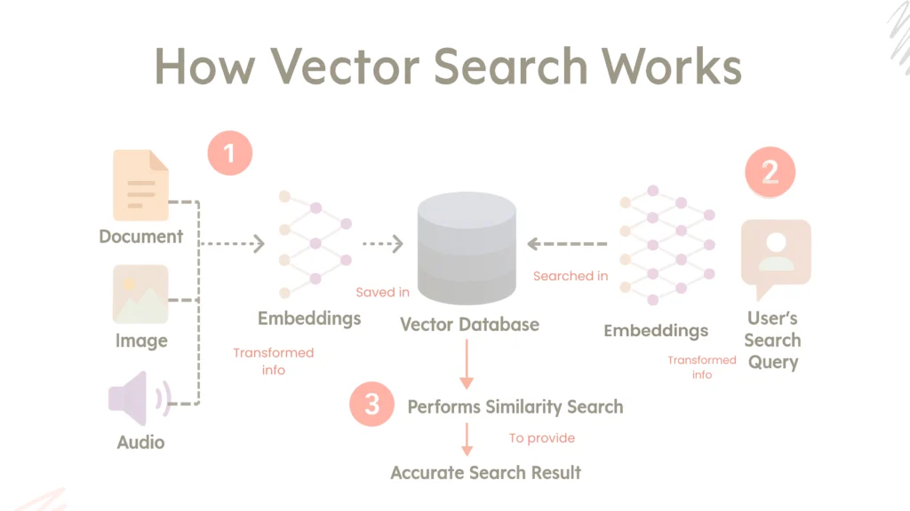
Vector search systems form the backbone of many AI and machine learning-based applications. Especially in areas like recommendation systems, semantic search, and image recognition, contents are indexed by converting them into high dimensional vectors and compared based on similarity. However, as data size grows, this process becomes computationally intensive and demands more hardware resources.

Therefore, to optimize vector search, a three-layered approach should be followed:

1 – Efficient Preparation of Vector Data

Data quality directly affects search results. Well-structured vector data not only ensures more accurate results but also enables more efficient use of system resources.

Normalization

Problem
Vectors with different magnitudes do not produce meaningfulm results, especially when using similarity measures like cosine similarity. Unscaled data can lead to inconsistent similarity scores.

Methods
● L2 Normalization: Each vector is scaled to unit length by dividing it by its own L2 norm. This ensures all vectors are on the same scale, providing consistency in cosine similarity calculations.
● Min-Max Normalization: Vector components are scaled to a specific range (usually between 0 and 1). This method standardizes values across different scales.
● Z-Score Normalization (Standardization): The mean is subtracted from each component, and the result is divided by the standard deviation. This results in a distribution with a mean of 0 and a standard deviation of 1. Especially useful for statistical modeling.
● Batch Normalization: Activations in a neural network layer are normalized based on the mean and variance within a mini batch. This accelerates training and increases stability.

Dimensionality Reduction

Problem

High-dimensional vectors (e.g., 1024 dimensions) require more computation and memory.

Methods

● PCA (Principal Component Analysis): A statistical dimensionality reduction technique that extracts principal components which best explain the variance in high dimensional data. It identifies axes carrying the most information and creates a new subspace accordingly. This reduces computational cost and noise.
● Autoencoder: An unsupervised neural network architecture that compresses high-dimensional data into compact and meaningful representations. It consists of an encoder and decoder. The encoder compresses the input into a lower-dimensional latent space, and the decoder attempts to reconstruct the original input. This process learns core features of the data.

In our project, embeddings obtained from language models (usually with 768 or more dimensions) are first passed through an autoencoder to reduce their size. For example, a 768 dimensional embedding is reduced to a 128-dimensional latent vector using the encoder. This smaller but semantically rich vector is then added to the vector database (e.g., Qdrant).

Advantages: Reduced computational cost, faster queries, and smaller index size.

Quantization

Problem

By default, vectors are stored as 32-bit floats, which consume large memory and disk space.

Methods

● 8-bit Quantization: Each vector component is represented as an 8-bit integer instead of a 32-bit float.
This reduces data size to one-fourth, significantly saving on storage and
computation.
● 16-bit Float (Float16) Quantization: Data is stored in 16-bit float format instead of 32-bit, halving data size while
preserving most of the accuracy due to float’s flexible range.
● Bfloat16 Quantization: A variant of 16-bit float with an 8-bit exponent that provides a wider value range.
Used in deep learning for faster computation with minimal accuracy loss.
● Int16 Quantization: Each vector component is stored as a 16-bit signed integer. Reduces data size by half and arithmetic is usually performed with 32-bit integers.
● Product Quantization (PQ): Vectors are split into segments (e.g., a 128-dimensional vector into 8 segments × 16 dimensions).
Each segment is compressed using its own codebook.
This provides huge memory savings and enables faster similarity comparison using code-level lookups.
Advantages: 70–90% storage savings, smaller index sizes, and significantly faster search performance.

2 – Using the Right Algorithms

Approximate Nearest Neighbor (ANN) Algorithms

Brute-force comparison with all vectors is not practical for large datasets. ANN algorithms provide huge speed gains with minor accuracy trade-offs. There are several variants:

Variant 1 – IVF (Inverted File Index)

Structure: IVF uses a clustering-based structure where vectors are grouped into predefined clusters. Each cluster contains a posting list of its closest vectors.

Working Principle: In the first step, the vector space is clustered using algorithms like k-means. Each vector is assigned to its nearest centroid. During query time, the search is conducted only within the nprobe closest clusters, which speeds up the process.

Parameters
● k: Number of clusters – determines granularity and index accuracy.
● nprobe: Number of clusters to search – higher values yield better accuracy but increase query time.
● PQ: Can be used with IVF to compress the memory footprint.

Advantages
● High Scalability: Capable of handling billions of vectors.
● Disk-based Execution: Ideal for data that doesn’t fit in memory.
● Performance-Oriented: Works efficiently especially for static datasets.
● FAISS Integration: IVF can be used efficiently via Facebook’s FAISS library.

Use Cases
● Visual similarity search
● Recommendation engines
● Large-scale AI systems

Limitations
● Limited dynamic data support – adding new data often requires re-clustering.
● Clustering quality directly affects performance.
● Poor clustering may miss close matches.

Variant 2 – HNSW (Hierarchical Navigable Small World)

Structure

HNSW organizes vectors into a multi-layered small-world graph. Each vector is a node connected to a number of neighbors. Higher layers have sparse, long-range connections; lower layers have dense, local ones.

Working Principle

Search begins at the top layer. The algorithm navigates to the closest node, then descends layer by layer for finer search. At the bottom, efSearch candidates are examined for best results.

Parameters
● M: Max number of neighbors per node – controls graph density.
● efConstruction: Number of candidates during indexing – higher value = better structure but longer build time.
● efSearch: Number of candidates during query – impacts accuracy and latency.

Advantages
● High accuracy: Despite being approximate, results are often near-exact.
● Low latency: Ideal for real-time systems.
● Dynamic: New vectors can be added without re-building.
● RAM-optimized: High-speed in-memory search.

Use Cases
● Real-time recommendation systems
● Dynamic content feeds
● High-accuracy information retrieval

Limitations
● High memory usage – resource-intensive on large datasets.
● Long index build time with high efConstruction.
● Inefficient for disk-based operations; RAM-dependent.

Variant 3 – ANNOY (Approximate Nearest Neighbors Oh Yeah)

Structure

ANNOY uses multiple binary tree structures based on random projections. Each tree divides vectors by projecting them onto random planes.

Working Principle
During indexing, each tree splits vectors into two groups using random hyperplanes, continuing recursively until leaves are formed. During search, multiple trees are queried, and search_k nodes are examined for best matches.

Parameters
● f: Vector dimension
● n_trees: Number of trees – affects accuracy and index size
● search_k: Number of candidates during query – balances accuracy vs speed

Advantages
● Disk-compatible: Indexes can be stored on disk and accessed via mmap.
● Low memory: Supports shared access and doesn’t require full in-memory loading.
● Fast index loading: Quick startup with mmap.
● Ideal for static datasets.

Use Cases
● Music recommendation systems like Spotify
● Embedding archives and vector search
● Index sharing in parallel systems

Limitations
● No update support – dynamic data requires full re-indexing.
● May perform poorly on high-dimensional sparse data.
● Generally lower accuracy than HNSW.

Other Alternatives

● ScaNN (Google): High accuracy with re-ranking and quantization support.
● DiskANN (Microsoft): Efficient for billions of vectors stored on disk.
● NMSLIB: Open-source, high performance, HNSW-like structure.

3 – Optimizing Infrastructure and Hardware

The speed and scalability of vector search systems are not only dependent on data and algorithms but also on infrastructure choices.

Distributed Systems and Sharding

Problem
A single server cannot handle billions of vectors.

Solution
The dataset is split into shards and distributed across multiple servers.

Parallel Querying
Each shard handles the query independently, and results are merged centrally.

Example Platforms
● Milvus: GPU-enabled, high-performance vector database
● Qdrant: Rust-based, fast, supports JSON filtering
● Vespa: Unified platform for vector search, filtering, and ML scoring
● Weaviate: Automatic embedding, semantic search, GraphQL support

GPU Acceleration

Problem
CPU-based search can result in high latency.

Solution
Parallel query processing using GPUs.
● FAISS-GPU: CUDA-based version of Facebook’s FAISS enables querying millions of vectors in milliseconds.

Performance Monitoring and Tuning

Metrics
● Recall@k: Is the correct result among the top k?
● Latency: Average query time
● QPS: Queries per second
● efSearch, nprobe: Parameters for balancing speed and accuracy
Also, hybrid search combines vector similarity with structured filtering for more targeted results.
Example: “Find similar images, but only from electronics category and priced below 500 TL”.
● Vespa: Combines ML scoring with classic filtering
● Qdrant: Supports powerful JSON-based filters
● Weaviate: Simple and flexible hybrid queries via GraphQL

Conclusion: Three-Layer Optimization Strategy

● Algorithm Level: Fast and flexible search with methods like HNSW and IVF
● Data Preparation Level: Efficient representation through normalization, dimensionality reduction, and quantization
● Infrastructure Level: Sharding, GPU acceleration, monitoring, and hybrid queries

When these layers are optimized together, it’s possible to achieve accurate results within milliseconds — even across datasets with billions of items.